Appendix D — Methodological Details

D.1 Survey Weighting

D.1.1 Building-Level Base Weights

Because Enumeration Areas (EAs) and building footprints were sampled prior to the commencement of fieldwork, it is possible to calculate a so-called base weight at the building level that represents how many other buildings each sampled building represents (including itself).

Building-level base weights are calculated as the inverse of the product of the probabilities of selecting each building \(j\) and each EA \(i\). Specifically, the building base weight \(d_{j}\) for the \(j\)th building is defined as

\[ \tag{building-level base weight} d_{j} = \frac{1}{\pi^{(1)}_{i} \times \pi^{(2)}_{j}} \]

where:

• \(\pi^{(1)}_{i}\) is the stage-1 probability of selecting the \(i\)th gridded EA in stratum \(h\) (note that for the sentinel sample, this is effectively 1).
• \(\pi^{(2)}_{j}\) is the stage-2 probability of selecting the \(j\)th building footprint,¹

D.1.2 Post-stratification of building weights

Using data on the degree of urbanization and other morphological features from the Global Human Settlement Layer (GHSL), these attributes are spatially joined to the entire sampling frame of all 2,420,103 building footprints in the sampling frame. The building-level base weights \(d_j\) then post-stratified to a new weight vector \(d^{\textrm{ps}}_j\) by Local Government Area (LGA) and GHSL feature to improve the representativeness of the weights.

D.1.3 Adjustment for Unknown Building Eligibility

Buildings are eligible if they are deemed residential. Whereas this is often easy to determine, there are some cases where the field team cannot establish the status of a sampled building. The building-level base weights are therefore adjusted to account for buildings where eligibility could not be determined (e.g., vacant or inaccessible). This adjustment was based on two stratum-level metrics, both displayed in Table D.1:

• the building completion rate for stratum \(h\), defined as the proportion of sampled buildings with completed interviews,
• the building known eligibility rate for stratum \(h\), defined as the proportion of sampled buildings for which eligibility status (i.e., building type) was known.

The product of these two quantities forms an adjustment factor \(a_h\). This factor is used adjust the post-stratified building weights:

\[ \tag{building-level adjusted weight} d^{\textrm{adj}}_{j \in q} = \frac{d^{\textrm{ps}}_j}{a_h} \] where

• \(q\) is the subset of sampled building footprints with known eligibility, and
• \(d^{\textrm{ps}}_j\) is the post-stratified weight for the \(j\)th building, and
• \(a_h\) is the known eligibility factor for stratum \(h\).

Table D.1: Building completion and known eligibility rates, by stratum

Stratum	Buildings Completed	Completion Rate	Known Eligibility Rate	Adjustment Factor
Gabasawa
1. Joda Ward	1,145	100%	100.00%	1.000
2. Tarauni Ward	771	100%	100.00%	1.000
3. Zugachi Ward	1,220	100%	100.00%	1.000
4. Mekiya Ward	1,908	100%	99.95%	0.999
5. Garun Danga Ward	1,519	100%	99.93%	0.999
6. Zakirai Ward	1,119	100%	100.00%	0.998
7. Gabasawa Ward	2,104	100%	99.95%	0.998
8. Yautar Kudu Ward	1,943	100%	99.85%	0.997
9. Yautar Arewa Ward	1,156	100%	99.91%	0.997
10. Karmami Ward	1,539	100%	99.87%	0.995
11. Yumbu Ward	809	99%	100.00%	0.993
Gaya
12. Gamarya Ward	712	100%	100.00%	1.000
13. Gaya South Ward	1,862	100%	100.00%	1.000
14. Kademi Ward	1,921	100%	99.95%	0.999
15. Shagogo Ward	1,842	100%	99.89%	0.999
16. Wudilawa Ward	846	100%	99.88%	0.999
17. Gaya North Ward	3,002	100%	99.93%	0.997
18. Maimakawa Ward	1,829	100%	99.78%	0.996
19. Balan Ward	1,184	100%	99.83%	0.995
20. Kazurawa Ward	1,215	99%	99.92%	0.991
21. Gamoji Ward	811	99%	99.88%	0.989
Nassarawa
22. Gwagwarwa Ward	229	100%	100.00%	1.000
23. Kaura Goje Ward	1,823	100%	100.00%	1.000
24. Hotoro North Ward	3,121	100%	99.97%	0.998
25. Hotoro South Ward	890	100%	99.78%	0.997
26. Gama Ward	826	100%	99.64%	0.996
27. Gawuna Ward	365	99%	100.00%	0.995
28. Kawaji Ward	2,120	99%	99.86%	0.993
29. Tudun Murtala Ward	1,422	99%	100.00%	0.988
30. Dakata Ward	909	99%	99.89%	0.986
31. Giginyu Ward	2,936	97%	99.76%	0.970
32. Tudun Wada Ward	455	94%	99.78%	0.942
Non-sentinel LGAs
33. Gezawa LGA	1,287	100%	99.92%	0.999
34. Dawakin Kudu LGA	2,196	100%	99.91%	0.999
35. Ungogo LGA	3,148	100%	99.87%	0.998
36. Dambatta LGA	1,972	100%	100.00%	0.998
37. Takai LGA	1,626	100%	99.88%	0.998
38. Dawakin Tofa LGA	1,951	100%	99.74%	0.997
39. Bebeji LGA	1,512	100%	99.80%	0.997
40. Tudun Wada LGA	1,906	100%	99.95%	0.997
41. Kumbotso LGA	5,743	100%	99.76%	0.997
42. Tarauni LGA	1,399	100%	100.00%	0.996
43. Kiru LGA	2,268	99%	99.96%	0.993
44. Sumaila LGA	2,530	99%	99.96%	0.989

D.1.4 Adjustment for Non-Response and Multiplicity

Household-in-building weights are calculated as the inverse of the probability of selecting each household \(k\) within a building \(j\) and EA \(i\). Specifically, the calibrated household-within-building weight \(w^{\textrm{cal}}_{j,k \in r}\) is computed as

\[ \tag{household-in-building weight} w^{\textrm{cal}}_{j,k \in r} = \frac{d^{\textrm{adj}}_j}{\pi^{(3)}_{k} \times m_{k} \times \hat{\phi}_{k}} \]

where:

• \(r\) is the subset of sampled households that resulted in a successful interview (the so-called response set), and
• \(\pi^{(3)}_{k}\) is the conditional stage-3 probability of selecting household \(k\) within sampled building \(j\), and
• \(m_k\) is the number of building structures reported by the respondent \(k\) as belonging to its household \(k\), and
• \(\phi_k\) is the modeled response propensity of household \(k\) (see the section on non-response below).

D.1.4.1 Multiplicity

The adjustment \(m_k\) controls for the multiple potential paths of entry of a household into the final sample (so-called “multiplicity”). This can happen if a household has both a main house and, say, a barn for animals and a toolshed. In this example, the given household would have three pathways into the sample (\(m_k=3\)). If, by chance, two of the buildings were sampled, it would be represented by two rows of data each having 1/3 of the usual building weight. The net effect is that when producing aggregated estimates, this household would have 2/3 the weight of a comparable household without multiple buildings. In practice, this household would only be interviewed once, and the data copied across two rows. This is collapsed back to a one-row-per-household basis in a later adjustment step described below.

D.1.4.2 Unit Non-Response

To reduce the impact of non-response bias, such as effects potentially arising from differences in skill between enumerators, Mindset built a series of multilevel logistic regression models and used the predicted probabilities to adjust survey weights. These models included a contact model and a cooperation model, whose predicted probabilities form the estimated response propensity for each household when multiplied together. The adjustment procedure assumes that non-response is conditionally independent after modeling. Models were fit on a random training subset of 70% of data collected for the conventional and adaptive components.² The formulas for these models are shown below using the notation from the {lme4} statistical package in R (Bates et al. 2025).

The contact model estimates the probability that an individual answers the door. It includes fixed effects for the interview time of day, the GHSL Morphological Settlement Zone (MSZ) layer, and the GHSL Global Human Settlement Layer Settlement Model (SMOD) layer (Pesaresi et al. (2023); Florczyk et al. (2019)). ghsl_msz is a categorical variable that characterizes the physical structure of an area. It captures attributes such as the height of residential buildings or whether a given building footprint is in a largely unbuilt area. The ghsl_smod variable is a categorical factor capturing the degree of urbanization. It takes values of mostly uninhabited, dispersed rural, village, semi-dense town, dense town, suburban or peri-urban, or city.

Additionally, random intercepts were included for LGA, ward, cluster, and subcluster (nested within each other), as well as for each field enumerator conducting the interview and field supervisor. For the non-sentinel area, the cluster variable represents the gridded EA, whereas in the sentinel area it is a custom cluster fit post-sample draw that assembled roughly 99 footprints per cluster for logistical purposes. The subcluster is a sub-division of the cluster that roughly partitions the cluster into three areas so that a team of three enumerators may divide the fieldwork amongst themselves.

NoteContact Model

lme4::glmer(
      formula = successful_contact ~ (1|lga_name/wardname/cluster/subcluster) + interview_time_of_day + ghsl_msz + ghsl_smod + (1|enumerator_id) + (1|supervisor_id),
      family = "binomial"
    )

The cooperation model estimated the probability that an eligible household with an infant aged 0–23 months would agree to participate. As in the contact model, it includes fixed effects for the interview time of day and for the GHSL Settlement Typology.

The model also includes random intercepts for LGA and ward (nested within the LGA), as well as for each enumerator and supervisor.

NoteCooperation Model

lme4::glmer(
  successful_cooperation ~ (1|lga_name/wardname) + interview_time_of_day + ghsl_smod + (1|enumerator_id) + (1|supervisor_id), 
  family = "binomial"
)

The summary of these models is presented below:

Table D.2: Regression coefficients

		(Model 1.1) Successful HH Contact	(Model 1.2) Successful Cooperation
Random Effects
σ²	Residual logistic variance	3.29	3.29
τ₀₀	LGA	0.06	0.04
	Ward within LGA	0.11	0.15
	Cluster within ward	0.23	0.50
	Subcluster within cluster	0.19	—
	Enumerator	0.42	0.69
	Supervisor	0.02	0.06
Observations		41,594	20,843
Marginal R² / Conditional R²		0.042 / 0.271	0.022 / 0.320

The \(\tau_{00}\) values represent the variance attributable to group-level random effects on the logistic scale (such as differences across LGAs or field staff) after accounting for the fixed effects.

The marginal \(R^2\) indicates the proportion of variance explained by the fixed effects alone, while the conditional \(R^2\) reflects the total variance explained by the full model, including both fixed and random effects. The gap between these two values measures the contribution of group-level structure to explaining response outcomes.

The residual latent variance \(\sigma^2\) is fixed at \(\pi^2/3 \approx 3.29\) by convention in multi-level logistic regression models.

In Table D.2, the low marginal \(R^2\) values suggest that the fixed effects account for only a small portion of variation in contact and cooperation, whereas the much higher conditional \(R^2\) values indicate that most of the explained variance comes from differences between groups captured by the random effects.

Assuming that contact and cooperation are conditionally independent given the model covariates, the predicted probability of response for each sampled household \(k\) in the set \(r\) of complete interviews, \(\hat{\phi}_k\), is then calculated as

\[ \hat{\phi}_{k\in r} = \hat{\nu}_k \hat{\gamma}_k \]

where \(\hat{\nu}_k\) is the predicted probability that the household was contacted (from the contact model), and \(\hat{\gamma}_k\) the predicted probability that the household agreed to participate once contacted (from the cooperation model).

Figure D.1: Calibration plots for the contact and cooperation models. Raw model probabilities are evaluated on a separate split of the data not use for training. 90% confidence ribbons shown.

(a) Contact Model

(b) Cooperation Model

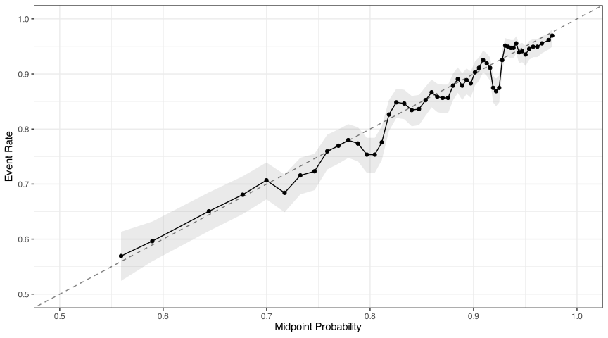
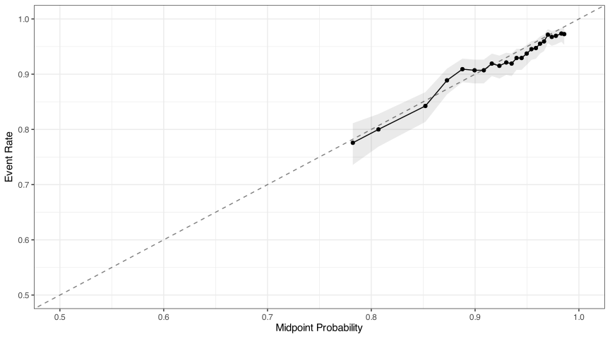
Before using these predicted probabilities to adjust the design weights, their calibration was checked using separate validation data splits. Calibration plots for both the contact and cooperation models compare the predicted probabilities to actual event rates across bins (Figure D.1).

The plots indicate that both models are reasonably well-calibrated in the regions most relevant to the observed data, supporting their use in non-response adjustment. The contact model achieved a Brier score³ of 0.12 and a Area Under the Receiver Operating Characteristic Curve (AUC-ROC)⁴ of 0.68, while the cooperation model performed slightly better with a Brier score of 0.08 and a AUC-ROC of 0.72 . These model scores were calculated on a partition of the data not used for model training .

After these checks, the predicted probabilities were used to adjust the design weights for non-response by dividing each unit’s weight by its corresponding \(\hat{\phi}_{k \in r}\). This increases the weight of respondents with lower estimated response probability and decreases it for those with higher response probability, helping to correct for non-response bias.

D.1.5 Weight Marginalization

Under the above design, certain households with multiple buildings footprints can be sampled more than once (hence the double-indexing \(w^{\textrm{cal}}_{j,k}\)). Although in practice, enumerators would only interview a repeated household once, these cases would have two or more rows of data in the original sample of building footprints. Therefore, in calculating household weights, weights \(w^{\textrm{cal}}_{j,k}\) are marginalized over distinct building footprints so that each row of data represents one household (without repeats). This produces a weight vector \(w^{\textrm{cal}}_{k}\) where each row represents a unique household.

D.1.6 Weight Trimming

To limit the influence of very large weights, weights \(w^{\textrm{cal}}_{k}\) were trimmed per LGA by capping them at 3.5 times the median LGA weight. This trimming step produces the new weight \(w^{\textrm{trim}}_{k}\) that helps limit the influence of individual units with very low response probabilities and results in more stable estimates that typically reduce the mean squared error of estimates. This procedure iteratively re-allocates some of the mass from large weights and redistributes it evenly to smaller weights such that \(w^{\textrm{trim}}_{k}\) sums to the same total as the untrimmed weight (\(\sum w^{\textrm{cal}}_{k} = \sum w^{\textrm{trim}}_{k}\)).

D.1.7 Expansion to Child-Level Weights

In principle, 100% of children 0-23 months were interviewed within sampled households that agreed to participate in the survey. For this reason, the stage-4 sampling probability is 100% and the child-level weights are effectively identical to their corresponding household level weight. For example, a given household that has a weight of 15.0 and twins would have child-level weights of 15.0 for each of the twins.

D.2 Variance Estimation

Estimates of Standard Errors (SEs) were produced using a generalized bootstrap method (Rao-Wu-Yue-Beaumont) (Beaumont and Émond 2022) as implemented by the {svrep} R package (Schneider 2025). This approach accounts for the complex multi-stage sampling design, which involved differing stratification levels, finite population correction, and sampling stages for sentinel and non-sentinel LGAs. All weighting adjustments applied to the main survey weight were also applied to the replicate weights. Several factors motivate the use of bootstrap weights over the simpler linearization variances. First, the bootstrap weights harmonize the two sampling designs (sentinel and non-sentinel) into a unified framework that is easy to analyze jointly. Second, they allow for post-stratification and calibration at different stages of sampling– something which is typically not supported by survey software. Since recent and precise population data is available at the level of building footprints, but not necessarily at the level of households, this flexibility enables post-stratification by the research team. Third, bootstrap weights make it simple to share replicate weights with third-party researchers, thereby allowing them to obtain the same variance estimates as Mindset without needing to have access to potentially sensitive design variable and/or without needing deep knowledge of the sampling design and sampling theory. Finally, the bootstrap weights also allow for the uncertainty associated with the unknown number of children to be reflected in the estimates, and for finite population corrections to be carried through in domain estimates. Most survey software drop finite population corrections on sub-domains that are not strata.

A set of 3,000 bootstrap replicate weights were generated. The first 500 are used in this report for analysis. The recommended number of bootstrap replicates depends on the amount of Monte Carlo error analysts are willing to accept, with larger numbers requiring more time and computation. This error is in addition to the sampling error, but can be made arbitrarily small by increasing the number of replicates used. Table D.3 estimates the number of replicates needed to keep the Monte Carlo error below a specified target for given variables of interest. For example, if we estimate the prevalence of zero-dose children using the Penta-1 approach, and we wish the variance of the estimates to be no more than 5% of the linearized estimate, then we would need 302 replicates. By the delta method, the relative Monte Carlo error on the standard error would be roughly half of that for the variance. This implies that with 302 replicates, we would expect roughly 2/3 of such bootstrap samples to have Monte Carlo error on SEs of 2.5% or less when estimating the Penta-1 zero-dose rate.

Table D.3: Expected number of replicate weights needed to reduce the Monte Carlo error down to a specified target level

Target coefficient of variation on the variance estimate	Suggested number of replicates to use	True zero-dose children (crude basis)	Penta-1 zero-dose children (crude basis)	Fully-vaccinated children (crude basis)
For estimating a proportion
0.01	14,286	14,286	7,534	9,926
0.02	3,572	3,572	1,884	2,482
0.03	1,588	1,588	838	1,103
0.04	893	893	471	621
0.05	572	572	302	398
0.10	143	143	76	100
For estimating a total
0.01	14,372	14,372	7,609	10,288
0.02	3,593	3,593	1,903	2,572
0.03	1,597	1,597	846	1,144
0.04	899	899	476	643
0.05	575	575	305	412
0.10	144	144	77	103

All analyses were conducted after applying the replicate design. This ensures that resulting SEs appropriately reflect the uncertainty associated with both the sampling design and the estimation of population sizes.

Bates, Douglas, Martin Maechler, Ben Bolker, and Steven Walker. 2025. Lme4: Linear Mixed-Effects Models Using Eigen and S4. https://github.com/lme4/lme4/.

Beaumont, Jean-François, and Nelson Émond. 2022. “A Bootstrap Variance Estimation Method for Multistage Sampling and Two-Phase Sampling When Poisson Sampling Is Used at the Second Phase.” Stats 5 (2): 339–57. https://doi.org/10.3390/stats5020019.

Florczyk, Aneta J., Christina Corbane, Daniele Ehrlich, Sergio Freire, Thomas Kemper, Lorenzo Maffenini, Michele Melchiorri, et al. 2019. “GHS Settlement Model grid (GHS‑SMOD), Global Human Settlement Layer Data Package 2019 (GHS P2019).” EUR 29788 EN (JRC 117104). European Commission, Joint Research Centre (JRC). https://doi.org/10.2760/290498.

Pesaresi, Martino, Marcello Schiavina, Panagiotis Politis, Sergio Freire, Kai Goch, Jürgen H. Uhl, Alessandro Carioli, et al. 2023. “GHS‑BUILT‑C R2023A: Morphological Settlement Zone (MSZ) dataset.” European Commission, Joint Research Centre (JRC). https://data.europa.eu/89h/3c60ddf6-0586-4190-854b-f6aa0edc2a30.

Schneider, Ben. 2025. Svrep: Tools for Creating, Updating, and Analyzing Survey Replicate Weights. https://bschneidr.github.io/svrep/.

---

1. For the non-sentinel sample, this is the conditional probability of sampling building \(j\) within the \(i\)th selected EA. For the sentinel sample, it is the unconditional stage-1 probability of selecting a building within stratum \(h\), since no actual sampling of EAs took place in the non-sentinel sample. For greater simplicity, this is harmonized into a single notation as \(\pi^{(2)}_{j}\). These building-level weights are calculated prior to data collection for all 77,807 building footprints sampled.

2. Combining data across the conventional and adaptive samples for model fitting allowed each survey component to borrow strength from the other by using a single model model to serve the non-response adjustment in each sample. Because the adaptive component has considerably smaller sample sizes, this pooling of information greatly improves the quality of the predicted response propensities.

3. The Brier score is a measure of how good a binomial model’s predicted probabilities are at describing the true frequency of an outcome. It is a so-called proper scoring rule, meaning it encourages honest probability estimates. For example, if a model produces quality predicted probabilities, then cases labelled as having 0.7 probability should actually occur 70% of the time. Brier scores closer to zero are better, with a max theoretical (bad) score at 0.25 when positive and negative classes have 50/50 balance.

4. The AUC-ROC metric measures how well a binomial model can distinguish between two outcome classes. If a model assigns higher predicted probabilities to true positives than to true negatives, it will have a higher AUC-ROC. An AUC-ROC of 0.5 indicates no discriminative ability (random guessing), while a score of 1.0 reflects perfect ranking of cases from highest to lowest risk. The AUC-ROC focuses only on ranking, not the calibration of predicted probabilities.