Variable | Type/Scale | Description | Encoding | MSA scorea |
|---|---|---|---|---|
urban | 0/1 | Place of residence | 1 urban; 0 rural | 0.952 |
toilet | ordinal 1–3 | Type of household toilet facility | 1 unimproved/other; 2 pit latrine; 3 flush toilet | 0.969 |
floor | ordinal 1–3 | Main flooring material used in the dwelling | 1 natural floor (earth / sand or dung); 2 rudimentary floor (wood plank or palm / bamboo); 3 finished floor (parquet or polished wood, vinyl or asphalt strips, ceramic tiles, cement, carpet | 0.939 |
walls | ordinal 1–3 | Main exterior wall material of the dwelling | 1 natural (cane / palm / trunks or dirt) or no walls; 2 rudimentary walls (mud, stone, uncovered adobe, plywood); 3 finished walls (cement, bricks, covered adobe, wood planks/shingles) | 0.825 |
roof | ordinal 1–4 | Main roofing material of the dwelling | 1 none; 2 natural (thatch, palm leaf, sod); 3 rudimentary (mat, bamboo, wood, cardboard); 4 finished (metal, cement fibre, tile, shingle) | 0.799 |
edu | ordinal 1–4 | Highest level of education attained by the respondent | 1 none/never; 2 primary; 3 secondary; 4 higher | 0.964 |
freqradio | ordinal 1–3 | Frequency of listening to the radio | 1 not at all; 2 less than once a week; 3 at least once a week | 0.857 |
freqtv | ordinal 1–3 | Frequency of watching television | 1 not at all; 2 less than once a week; 3 at least once a week | 0.916 |
has_phone | ordinal 1–3 | Ownership or access to a mobile or household phone | 1 none/unknown; 2 household phone (non-smart); 3 smartphone | 0.939 |
internet | ordinal 1–3 | Frequency of internet access | 1 has never used; 2 uses less than daily; 3 uses internet daily | 0.933 |
has_elec | 0/1 | Household has access to electricity | 1 yes | 0.962 |
has_radio | 0/1 | Household owns a radio | 1 yes | 0.873 |
has_tv | 0/1 | Household owns a television | 1 yes | 0.906 |
has_fridge | 0/1 | Household owns a refrigerator | 1 yes | 0.948 |
own_watch | 0/1 | Household member owns a wristwatch | 1 yes | 0.955 |
own_computer | 0/1 | Household owns a desktop or laptop computer | 1 yes | 0.936 |
own_motorcycle | 0/1 | Household owns a motorcycle or scooter | 1 yes | 0.884 |
own_car | 0/1 | Household owns a car or truck | 1 yes | 0.880 |
own_dwelling | 0/1 | Household owns its dwelling unit | 1 yes | 0.870 |
own_land | 0/1 | Household owns agricultural or residential land | 1 yes | 0.931 |
livestock | count | Number of livestock owned by the household | non-negative integer | 0.679 |
herds | count | Number of large herds (e.g., cattle, camels) owned | non-negative integer | 0.723 |
poultry | count | Number of poultry owned | non-negative integer | 0.593 |
animals | count | Number of other animals (e.g., goats, pigs, etc.) owned | non-negative integer | 0.595 |
works | ordinal 1–3 | Employment status of the respondent | 1 not working/student/retired/unemployed; 2 self/part-time; 3 full-time | 0.901 |
fuel | ordinal 1–5 | Primary fuel used for cooking | 1 wood; 2 agricultural crop; 3 charcoal; 4 natural gas; 5 electricity | 0.963 |
hectares | numeric | Size of land owned in hectares | 0 none; 1 <1 ha; else numeric hectares | 0.653 |
aMeasure of sampling adequacy from the Kaiser-Meyer-Olkin test for factor adequacy | ||||
Appendix F — Wealth Index
The household wealth index was constructed using Principal Components Analysis (PCA), inspired by the approach used in the Nigeria Demographic and Health Survey (NDHS). This method, introduced by Rutstein and Johnson (2004) and detailed in subsequent technical notes on implementation (Rutstein 2008), provides a consistent, data-driven means of estimating relative household economic status from nonmonetary indicators. The approach has been further described in the Demographic and Health Survey (DHS) methodological documentation on data reduction and factor analysis (Rutstein 2015). It offers a practical alternative to direct measures of income or consumption, which are often difficult to obtain accurately in low-resource settings due to recall error, informal earnings, and respondent reluctance to disclose financial information. By summarizing asset ownership, housing quality, and access to basic services into a single composite measure, the PCA-based wealth index captures long-term economic capacity and allows for standardized quintile classification across populations. In this pipeline, the wealth index is estimated on the collapsed household interview dataset derived from completed child-module interviews. This means that quintile labels in this report are relative ranks within the study sampling frame (households with age-eligible children across the 15 study Local Government Areas (LGAs)), not national wealth quintile cut points for all households in Nigeria. As a result, Network Scale-Up Method (NSUM)-only interviews that do not have a completed child module are generally outside the estimation frame and therefore do not receive a wealth quintile.
Table F.1 lists the 27 variables used in this study for the household wealth index. Missing values were imputed using multivariate imputation by chained equations using the R {mice} package, drawing on imputation algorithms such as random forests, ordinal regression, logistic regression, and predictive mean matching. Where necessary, responses were transformed into consistent, directionally coherent indicators of household living standards—such that higher values consistently represent better housing, greater asset ownership, or improved access to services. Some inputs are ordinal variables, capturing ordered differences in quality or frequency (for example, education level, toilet type, or floor material), while others are binary (0/1) indicators representing simple ownership or presence (for example, electricity, radio, or refrigerator).
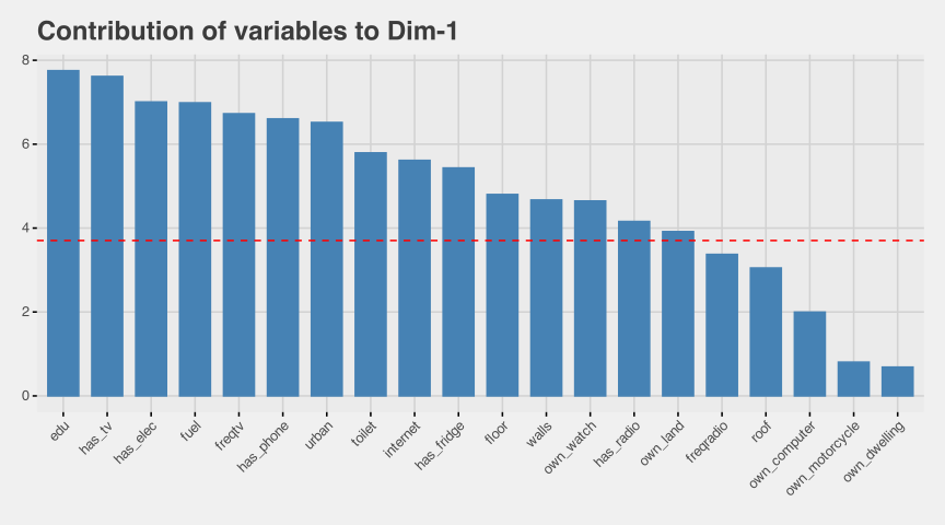
Diagnostics indicated that the PCA was appropriate. Bartlett’s test of sphericity showed that the correlation matrix differed significantly from the identity matrix, \(\chi^2(351) = 1.6058\times 10^{5}, p<0.001\), confirming sufficient intercorrelations among variables to justify principal component analysis. The Kaiser–Meyer–Olkin (KMO) measure of sampling adequacy was high, with an overall Measure of Sampling Adequacy (MSA) of 0.92 (excellent), and individual items ranging from 0.59 to 0.97 (shown in Table F.1). Together, these diagnostics indicate that the data are well suited for PCA. The first principal component–used as the wealth index–explains 26% of the total variance in the input variables. Figure F.1 shows the top 20 variables that contribute to the wealth index.
The factor loading plot in Figure F.2 shows a clear socioeconomic gradient along the first principal component, which serves as the constructed wealth index. Variables associated with higher living standards—such as ownership of durable goods (television, refrigerator, car, computer) and improved housing materials (cement floors, brick walls, access to electricity)–load strongly and positively on this dimension. Conversely, indicators of deprivation or subsistence living, including use of natural or rudimentary building materials, reliance on basic fuels, and ownership of livestock or poultry, load negatively. This pattern confirms that the first component captures a coherent continuum from poorer to wealthier households. The second dimension distinguishes households more by context than by wealth: urban-related indicators (internet access, modern appliances, smaller livestock ownership) load in one direction, while rural markers (ownership of animals, land, and use of traditional fuels) load in the opposite. This is also shown in Figure F.3, which shows the joint loadings of the variables on the first two components. Together, the first two components suggest that economic well-being is the dominant source of variation, with an orthogonal axis separating rural and urban forms of livelihood. The plot thus reinforces the interpretive validity of the first component as a reliable wealth index within this population.


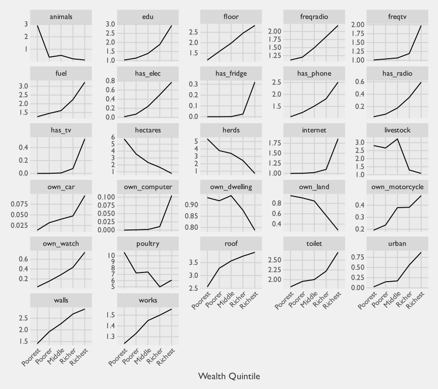
Finally, we can turn to Figure F.4 validate that the PCA-derived wealth index tracks expected patterns for the population along wealth quintiles. Using weighted survey estimates, we see that across almost all indicators, the expected monotonic relationships with wealth quintiles are evident: ownership of durable goods, access to electricity, improved sanitation, higher education, and better housing materials increase consistently from the poorest to the richest groups. In contrast, markers of rural or subsistence living—such as ownership of livestock, poultry, or agricultural land—decline with wealth, reflecting structural differences in livelihood patterns.
Because these results are based on design-weighted data, they demonstrate that the wealth index not only orders households coherently within the sample but also reflects meaningful socioeconomic stratification in the target population. The generally monotonic increase in a variable’s wealth/quality across quintiles, along with the consistent direction of associated indicators, provides strong evidence of the construct validity of the index as a population-representative measure of material well-being.